Context Link to heading
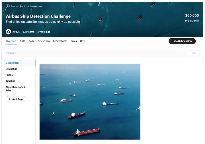
In 2018, when I was still working at Airbus Defence and Space, I organised a challenge on Kaggle to detect ships in Airbus SPOT satellite imagery (@ 1.5 meters resolution).
Check my article about the successes and issues that we encountered. That’s a whole story in itself!
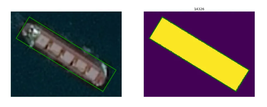
One of the interesting characteristics of the challenge was the oriented bounding boxes annotations. When we annotated the dataset, we decided to create rotated rectangles to closely fit the ships that we saw on the imagery. Intuitively, we thought that classic bounding boxes were including too much background. Of course, this was not perfect as well for small speed boats which we could not clearly separate from their wake.
But at the time, there was very little literature about oriented bounding boxes. So the Kaggle team decided to encode our rectangle bounding boxes into RLE which is a format suited for creating binary masks. And actually most teams used deep learning architectures suited to mask prediction. I will analyse the best practices for segmentation used by the participants and described on Kaggle forums. And then present a completely different approach based on new oriented bounding box architectures.
Analysis of winner solutions in 2018 Link to heading
But before developing a segmentation model to identify the ships, the participants needed to overcome a first problem of unbalanced classes.
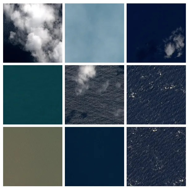
The sea is mostly void of ships. And waves or clouds can look like small ships on a satellite image. So we wanted the dataset to include some images of sea without any ships and with various conditions of weather and sea formation.
But, unfortunately, the way we generated the imagery created a LOT of images with no ships ; actually out of 231,723 imagery extracts of 768 x 768 pixels, only 81,723 had ships on them. Models usually do not like to be trained on too many empty images, so it made sense to reduce the number of empty images during the training.
But if the segmenter had not seen a lot of empty images during training, this meant that it would be prone to over-detection during inference. So most of the participants created a two stage detector with first a classifier and then segmenter. The purpose of the classifier was to detect if the image was likely to contain ships and only send these likely images to the segmenter.
The other reason to create a classifier was that the chosen metric for scoring participants was very biased against detecting a single ship when there was none. This in itself will be the subject for another post. It definitely pushed participants to create this two-stage detector.
This is not a bad thing because classifiers are much faster then segmentation models and, as I said earlier, sea is mostly void of ships — so this means that the detector was going faster on vast areas of open sea.
First step : Ship <> No Ship Classifier Link to heading
Training a good Ship <> No Ship classifier was more important for this competition than having a very good performing segmentation model. The objective was to fight fight false positives (bright spots, wave glare, etc). The classifier should, of course, to be as good as possible and to avoid classifying images with ships as images without ships. But note, that there is an asymmetry in this process: if an image with ship was classified without ship it was lost forever although an error in the other direction could potentially be corrected by the segmenter.
Back in 2018, the architectures selected for this task where mostly all flavours of ResNet (ResNet-18, ResNet-34, ResNet-50, ResNet-101 and ResNet-152) with some others like DPN-68, DPN-92 or DenseNet-121. A simple training of a ResNet-50 over 10 epochs leads to a 0.975 accuracy which was good but not enough to be in the top 3.
All the winners decided to train an «ensemble» of models for the classifier. Either by training different architectures or the same architecture on different split of the training data (using cross-validation). Then the results from the various models would just be summed and averaged.
Second step : Segmenter Link to heading
Segmentation models are neural networks which produces a mask from an input image. They are usually U-shaped and for this called U-Net. The left side of the U is the encoder which encode the semantic information while reducing the spatial dimension. Then, the right side of the U acts as a decoder to generate the mask containing the semantic information at the correct location. To make sure that the reconstruction is fine-grained, there are shortcuts connections from the encoding branch to the decoding branch to convey the spatial information which has been lost in the semantic encoding.
All winners used U-Net architecture with various backbones (i.e. encoders). Some participants used FPN architectures and other Mask-RCNN architectures (see below). Larger backbones are not always a must. Smaller architectures like ResNet-34 could work well if trained long enough.
Since that images where pretty large (768x768 pixels) to fit in large batches in the GPU memory, one smart trick was to use 256x256 crops, randomly selected around the center of the ships. Of course, resizing images was out of questions because it will make the small ships disappear.
Of course, since the dataset was unbalanced and had a lot of empty images, it was important to reduce number of images with no ships. But one should make sure not to remove them completely. A mix of 20% of images with no ships was important to help the model understand that this could be a normal situation. This could also be done by augmenting the images with ships compared to the images without ships.
Most participants used several U-Net either with different architecture or specialised on various tasks (like large ships and small ships). The final “ensembling” step was mostly to sum or average the various generated masks. In some case, TTA (or Test Time Augmentation) was also used. This means that the same image was sent to the model after being flipped and/or rotated. The results will then be averaged again.
You can check the following blog posts for the participants:
Final step : Post processing Link to heading
After the U-Net had produced a mask, the the last step was to vectorise this mask and create distinct polygons for each individual ship. But, in fact, to deal with ships which were docked side by side, an extra trick was necessary.
The exterior boundary of the ship had to be treated as a second class. Some participants also decided to treat the contact zone between two ships as a third class. In any case, the trick was to make sure to identify this area as it was key in being able to reconstruct the individual shape of each ship when they were side by side.
https://www.kaggle.com/competitions/airbus-ship-detection/discussion/71659
The rest of the processing is then done by using python Computer Vision like rasterio or ski-image. Using morphological tools like erosion and dilatation to remove objects under a specific threshold, using a convex hull function, creating an image of distance from border of objects, extracting local peaks or centroid, using watershed techniques and finally vectorisation.
One interesting technique was definitely to use pseudo-labelling. The dataset included a large number of unlabelled tiles which was designed to be used to test the model. Participants were expected to predict ships on the test dataset and submit the resulting predictions as RLE masks. But the predictions could also be used to further train the model and potentially increase slightly the performance of the model.
When all these steps were done the best possible way, it was possible to reach the highest score on the leaderboard. Typically above 0.854. Here is a nice video of how trials and errors can lead to an honorable submission.
Rotated rectangle or Oriented bounding boxes? Link to heading
Starting from vectorised annotations to generate masks, then using segmentation architectures to generate raster masks and finally vectorising the predicted masks to deliver oriented bounding boxes made a few participants explore other techniques.
Some participants were quite successful using Mask-RCNN although it was based on simple axis-aligned bounding boxes. Check the following Kaggle post.
At the time, we would also see the first papers on ArXiv about oriented bounding box architectures. The main idea was to add an extra parameter to the model to predict the orientation of the bounding box either as a discreet parameter or a continuous parameter. In the later case, there was some added complexity to the code as an angle is non-continuous between 359.99° and 0°.
At the time, a few participants experimented with oriented bounding boxes detector which seemed like a reasonable thing to do but they did not get very good results.
Let’s explore what we can do in 2023 in that respect!
How to get oriented bounding boxes annotation? Link to heading
Before being able to implement new type of solution, we need to have oriented bounding boxes annotations. And although Airbus created the annotation as rectangles, these are not available in the Kaggle dataset.
So we need to recreate them from the RLE encodings. Kaggle grandmaster iafoss created an new version of the dataset with oriented bounding boxes but, unfortunately, it is based on the original version of the dataset. Actually, there are two version of the dataset and only the last one is available. Check my previous post for a longer story about why this is the case.
Again we will be using some fantastic python packages like rasterio and shapely. Here is the code to convert RLE to oriented bounding boxes. You can check this Kaggle notebook to see it in action.
# convert RLE encoded pixels into binary mask
mask = encode_mask(str(row.EncodedPixels), shape=(768,768))
# vectorize mask into GeoJSON
value = 0.0
for polygon, value in list(features.shapes(mask)):
if value == 1.0:
break
if value != 1.0:
print('Error while vectorizing mask')
# get oriented bounding box around shape
coords = polygon['coordinates'][0]
obbox = MultiPoint(coords).minimum_rotated_rectangle
# get center of bounding box and correct for half a pixel
xc, yc = list(obbox.centroid.coords)[0]
xc, yc = xc - 0.5, yc - 0.5
# get external coordinates of oriented rectangle
# compute length, width and angle
p1, p2, p3, p4, p5 = list((obbox.exterior.coords))
dx = math.sqrt((p3[0] - p2[0])**2 + (p3[1] - p2[1])**2)
dy = math.sqrt((p2[0] - p1[0])**2 + (p2[1] - p1[1])**2)
angle = math.atan2((p3[1] - p2[1]), (p3[0] - p2[0]))
#length = max(d1, d2)
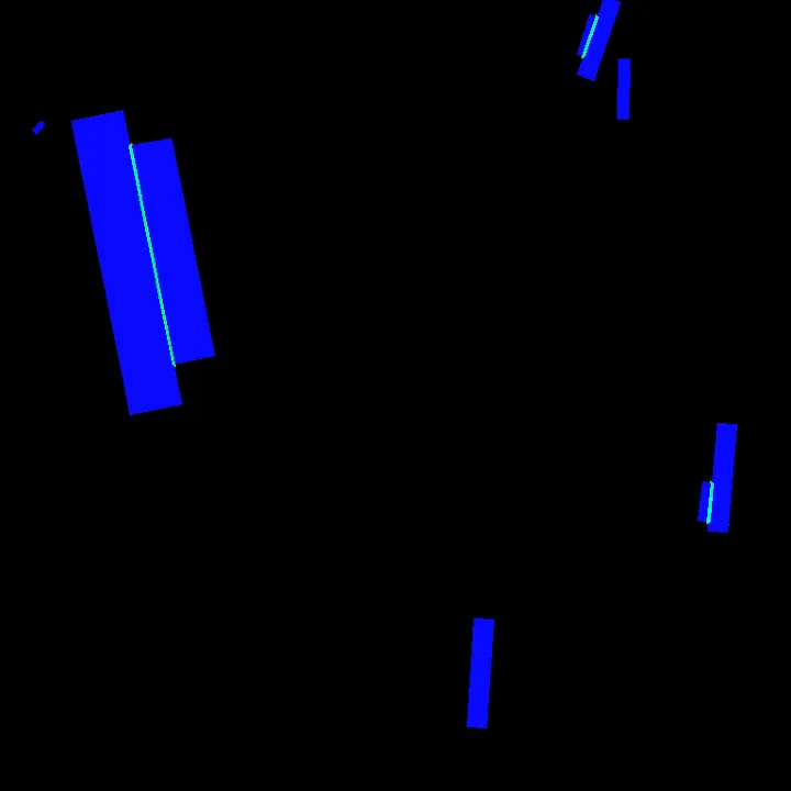
#height = min(d1, d2)Some examples to check for quality. The visualisation scripts are mostly based on iafoss work that you can found here.
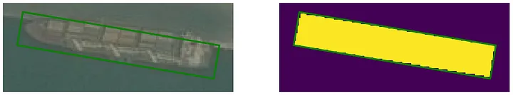
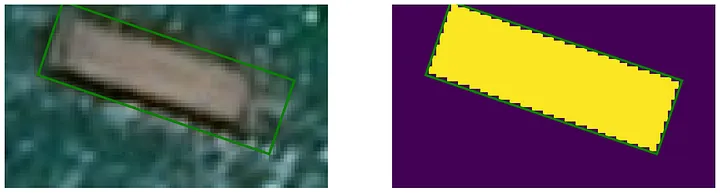
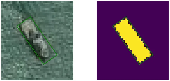
These examples show that although some ships are easy to detect, there are also many cases where the boundaries are not clear, the acquisition angle not vertical or the colour very similar to the sea colour.
Let’s now dive into a new fantastic framework to work with oriented bounding boxes detectors. It is called MMRotate from Open MMLab.
Introducing OpenMMLab and MMRotate Link to heading
In one of my previous post, I presented and used IceVision to test various model architectures on the same task. Another fantastic framework to experiment with various computer vision deep learning architectures is the OpenMMLab framework.
OpenMMLab is an open-source algorithm platform for computer vision. It aims to provide a solid benchmark and promote reproducibility for academic research. We have released more than 30 high-quality projects and toolboxes in various research areas such as image classification, object detection, semantic segmentation, action recognition, etc. OpenMMLab has made public more than 300 algorithms and 2,400 checkpoints. Over the past years, OpenMMLab has gained popularity in both academia and industry. It receives over 78,000 stars on GitHub and involves more than 1,700 contributors in the community.
The code base is available on GitHub and is organised in various independent task-specific packages which all rely on foundation libraries MMEngine for training loops, MMCV for computer vision functions and PyTorch as Deep Learning library.
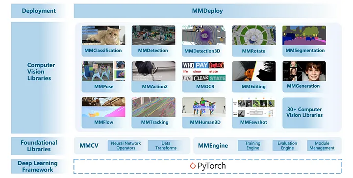
Aside MMDetection which offers model architectures and tools for standard bounding box detection, there a specific package for oriented bounding boxes which is called MMRotate.
The code was published and very actively updated one year ago in spring 2022. Recently the team has focused on introducing the MMEngine module which centralise the deep learning related code and reorganising the various modules accordingly.
Install the MMRotate package and its dependencies Link to heading
In the following code, we will stick with the version 0.3.4 from 2022. The corresponding documentation is here. Note that we make sure to install the corresponding MMCV and MMDet versions.
# Install MMCV and MMDetection
RUN pip install -U openmim
RUN mim install mmcv-full==1.7.1
RUN mim install mmdet==2.28.2

# Install MMRotate v0.3.4
RUN git clone --depth 1 --branch v0.3.4 https://github.com/open-mmlab/mmrotate.git
WORKDIR mmrotate
Create a custom Data Loader for our data Link to heading
A simple way to adapt the code to a specific use case is to convert the training data to the DOTA format as described here.
I usually like to preserve the source data as it is so that I can more easily manage multiple version of it. For MMRotate, this mostly involves creating a new Dataset Type and loading annotations directly from where they are stored. In our case, since the source annotation are provided as a CSV file, I am using a pandas DataFrame to read and store the annotations.
Here is the code that will help you create your own Dataset Type:
from mmrotate.datasets.builder import ROTATED_DATASETS, PIPELINES
from mmrotate.datasets.dota import DOTADataset
import glob
import numpy as np
import pandas as pd
from mmrotate.core import poly2obb_np
import os.path as osp
import os

from mmdet.datasets.pipelines import LoadImageFromFile
from PIL import Image

def convert_rbb2polygon(bbox):
    xc, yc, w, h, ag = bbox
    wx, wy = w / 2 * np.cos(ag), w / 2 * np.sin(ag)
    hx, hy = -h / 2 * np.sin(ag), h / 2 * np.cos(ag)
    p1 = (xc - wx - hx, yc - wy - hy)
    p2 = (xc + wx - hx, yc + wy - hy)
    p3 = (xc + wx + hx, yc + wy + hy)
    p4 = (xc - wx + hx, yc - wy + hy)
    poly = np.array([p1[0], p1[1], p2[0], p2[1], p3[0], p3[1], p4[0], p4[1]])
    return poly

def convert_rbb2polygons(bboxes):
    polygons = []
    for i, bbox in enumerate(bboxes):
        poly = convert_rbb2polygon(bbox)
        polygons.append(poly)
    return polygons

@ROTATED_DATASETS.register_module()
class AirbusShipDataset(DOTADataset):
    """Airbus Ship dataset for detection."""

    CLASSES = ('ship',)

    def load_annotations(self, ann_file):
        """
            Args:
                ann_folder: folder which contains the CSV file witn annotations
        """
        cls_map = {c: i
           for i, c in enumerate(self.CLASSES)
           }

        data_infos = []
        if not os.path.isfile(ann_file) :  # test phase
            img_files = glob.glob(self.img_prefix + '*.jpg')
            for img_file in img_files:
                data_info = {}
                img_id = osp.split(img_file)[1][:-4]
                img_name = img_id + '.jpg'
                data_info['filename'] = img_name
                data_info['ann'] = {}
                data_info['ann']['bboxes'] = []
                data_info['ann']['labels'] = []
                data_infos.append(data_info)
        else:
            box_df = pd.read_csv(ann_file)

            # parse all images
            for ImageId, ann_df in box_df.groupby('ImageId'):
                data_info = {}
                img_id = osp.split(ImageId)[1][:-4]
                img_name = ImageId #img_id + '.jpg'
                data_info['filename'] = img_name
                data_info['ann'] = {}
                gt_bboxes = []
                gt_labels = []
                gt_polygons = []
                gt_bboxes_ignore = []
                gt_labels_ignore = []
                gt_polygons_ignore = []

                if len(ann_df) == 0 and self.filter_empty_gt:
                    continue

                # parse all annotations in this image
                for row_index, row in ann_df.iterrows():

                    # read annotation
                    x, y, w, h, a = row['xc'], row['yc'], row['dx'], row['dy'], row['angle'],
                    label = cls_map['ship']

                    # add to lists of annotations for this image
                    gt_bboxes.append([x, y, w, h, a])
                    gt_labels.append(label)
                    poly = convert_rbb2polygon([x, y, w, h, a])
                    gt_polygons.append(poly)

                if gt_bboxes:
                    data_info['ann']['bboxes'] = np.array(
                        gt_bboxes, dtype=np.float32)
                    data_info['ann']['labels'] = np.array(
                        gt_labels, dtype=np.int64)
                    data_info['ann']['polygons'] = np.array(
                        gt_polygons, dtype=np.float32)
                else:
                    data_info['ann']['bboxes'] = np.zeros((0, 5),
                                                          dtype=np.float32)
                    data_info['ann']['labels'] = np.array([], dtype=np.int64)
                    data_info['ann']['polygons'] = np.zeros((0, 8),
                                                            dtype=np.float32)

                if gt_polygons_ignore:
                    data_info['ann']['bboxes_ignore'] = np.array(
                        gt_bboxes_ignore, dtype=np.float32)
                    data_info['ann']['labels_ignore'] = np.array(
                        gt_labels_ignore, dtype=np.int64)
                    data_info['ann']['polygons_ignore'] = np.array(
                        gt_polygons_ignore, dtype=np.float32)
                else:
                    data_info['ann']['bboxes_ignore'] = np.zeros(
                        (0, 5), dtype=np.float32)
                    data_info['ann']['labels_ignore'] = np.array(
                        [], dtype=np.int64)
                    data_info['ann']['polygons_ignore'] = np.zeros(
                        (0, 8), dtype=np.float32)

                data_infos.append(data_info)

        self.img_ids = [*map(lambda x: x['filename'][:-3], data_infos)]
        return data_infos
Configuration file Link to heading
MMRotate is all about configuration files as the other OpenMMLab components. You can certainly use MMRotate without but they are the best way to manage various experiments. The idea behind this is that all the parameters for your dataset, you model and your training loop are actually stored in a configuration file (as a Python dictionary or a YAML file).
This makes it very easy to compared parameters between two experiments (i.e. training of a model). This also enables you to start from one of the existing configuration files and just modify the parameters that you need. OpenMMLab provides a benchmark and model zoo page where you will find all the base configuration files that you can tweak to your needs.
For exemple, here, we select ReDet which is described in this paper: ReDet: A Rotation-equivariant Detector for Aerial Object Detection. The following code download the configuration file for the model with a ResNet-50 backbone, the training loop as well as the associated pre-trained weights on the DOTA dataset.
# We use mim to download the pre-trained checkpoints for inference and finetuning.
!mim download mmrotate --config redet_re50_refpn_1x_dota_ms_rr_le90 --dest .

CONFIG_FILE = 'redet_re50_refpn_1x_dota_ms_rr_le90.py'

cfg = Config.fromfile(CONFIG_FILE)
print(f'Config:\n{cfg.pretty_text}')
We need to make a few changes to this configuration file. We can copy and modify the file or we can make the changes programmatically to the configuration in memory. So we can use Python rather than YAML.
Here we define the source data:
# Change the dataset type from DOTADataset to AirbusShipDataset
cfg.dataset_type = 'AirbusShipDataset'

# Change the location of the root folder for training data
cfg.data_root = '/data/share/airbus-ship-detection/'

# Change the size of the image (instead of 1024 with DOTA)
cfg.img_size = 768

# Adapt the number of images accordingly with your GPU memory
cfg.data.samples_per_gpu=20

# Define the value for normalization
# This needs to be computed in the EDA
# MMRotate uses cv2 to read imagery so it expects BGR and not RGB
# Re-order the channels to RGB after normalization
cfg.img_norm_cfg = dict(
    mean=[52.29048625, 73.2539164, 80.97759001],
    std=[53.09640994, 47.58987537, 42.15418378],
    to_rgb=True)
And next, the data pre-processing:
cfg.train_pipeline = [
    # Read images from file with MMDet (cv2)
    dict(type='LoadImageFromFile'),
    # Read annotations. This is the function that we overloaded earlier
    dict(type='LoadAnnotations', with_bbox=True),
    # Resize to the initial size of the model
    # For satellite images, we want to avoid any downscaling
    dict(type='RResize', img_scale=(cfg.img_size, cfg.img_size)),
    # Define a 'flip' augmentation
    dict(
        type='RRandomFlip',
        flip_ratio=[0.25, 0.25, 0.25],
        direction=['horizontal', 'vertical', 'diagonal'],
        version='le90'),
    # Define a 'rotation' augmentation
    dict(
        type='PolyRandomRotate',
        rotate_ratio=0.5,
        angles_range=180,
        auto_bound=False,
        version='le90'),
    # Normalize the radiometry
    dict(type='Normalize', **cfg.img_norm_cfg),
    # Pad the image to be divisible by 32
    dict(type='Pad', size_divisor=32),
    # Return images, bboxes and labels as tensors
    dict(type='DefaultFormatBundle'),
    dict(type='Collect', keys=['img', 'gt_bboxes', 'gt_labels'])
]
Then, we initialise the training data source with our previous parameters: the dataset type, the dataset root, the train.csv file with train annotations and the train data pipeline.
cfg.data.train=dict(
    type=cfg.dataset_type,
    ann_file='train.csv',
    img_prefix='train_v2/',
    pipeline=cfg.train_pipeline,
    version='le90',
    data_root=cfg.data_root
)
We also need to tweak the final layers of the model because DOTA has 15 classes and we have only one class (for ships)
# modify num classes of the model in two bbox head
cfg.model.roi_head.bbox_head[0].num_classes = len(AirbusShipDataset.CLASSES)
cfg.model.roi_head.bbox_head[1].num_classes = len(AirbusShipDataset.CLASSES)
There are many more modifications that you can make, like modifying the learning rate, the learning rate policy, the anchor generator, etc… Here we just define the maximum epochs and the logging interval.
cfg.runner.max_epochs = 50
cfg.log_config.interval = 200
Finally, I like to organise the logs by architecture and date and I make sure to save the configuration file with the logs so that I can retrieve it later if needed.
# Get architecture name from config file name
config_name = os.path.basename(CONFIG_FILE)
keyname = config_name.split('_')[0]

# Get current time
now = datetime.datetime.now()
date_time = now.strftime("%Y-%m-%d-%H-%M-%S")

# Set up folder to save config file and logs
cfg.work_dir = os.path.join('./logs', keyname, date_time)

# Create folder
mmcv.mkdir_or_exist(os.path.abspath(cfg.work_dir))

# Save updated configuration file in logs folder
cfg.dump(os.path.join(cfg.work_dir, config_name))
Training Link to heading
After we have finished modifying the configuration file, the next step is to train the model.
from mmdet.models import build_detector
from mmdet.apis import train_detector

# Build the train dataset (and optionaly validation dataset)
datasets = [build_dataset(cfg.data.train)]

# Build the detection model
model = build_detector(cfg.model)

# Launch training
train_detector(model, datasets, cfg, distributed=False, validate=False)
After 20 epochs, the metrics (mAP) reaches a plateau and we can stop the training to display some outputs.
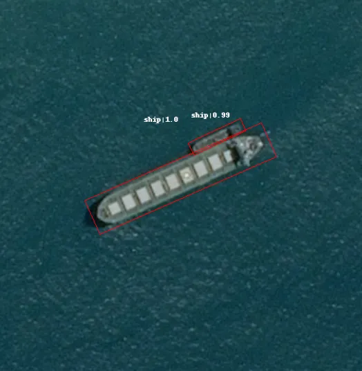
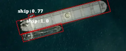
The models performs pretty well in most case and deals pretty well with ships close to each other. The models runs faster than UNet and delivers directly oriented bounding boxes.
Of course, this is not directly an exceptional model like the ones which were on top of the leaderboard. Some improvement points are:
- Add a classifier before the detector to remove false detections
- Modify the anchor generator to fit the specific shape of ships
- Add TTA (Test-Time Augmentation)
- Increase the dataset by doing pseudo-labelling on the test data
But globally it is very easy to apply MMRotate to this dataset and the OpenMMLab framework should have its place in most R&D work for object detection on satellite and aerial imagery.
Conclusion Link to heading
If you have not already experimented with OpenMMLab and MMRotate, I hope that this blog post will motivate you to test it. I am using it in many of my projects and I am impressed. It requires somewhat of a learning curve but it definitely worth it as it is a powerful yet flexible tool.
Written on November 16, 2023 by Jeff Faudi. Link to heading
Originally published on Medium