The latest YOLO version has been published Link to heading
YOLOv8 is the latest version of the YOLO object detection and image segmentation models developed by Ultralytics. YOLOv8 is a cutting-edge, state-of-the-art (SOTA) model that builds upon the success of previous YOLO versions and introduces new features and improvements to further boost performance and flexibility.
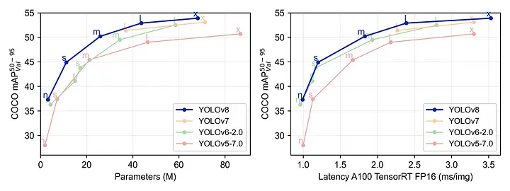
Performances of the YOLO series (source)
YOLOv8 is designed to be fast, accurate and user-friendly, making it a popular choice among researchers and practitioners in computer vision and AI. Ultralytics YOLOv8 provides pre-trained models, easy-to-use tutorials, and access to a community of experts to help users get started quickly.
In this article, we will explore how this new YOLO version can be used on satellite images — typically detecting aircrafts on Pleiades images.
The YOLO history Link to heading
YOLO (You Only Look Once) is a popular object detection and image segmentation model developed by Joseph Redmon and Ali Farhadi at the University of Washington. The first version of YOLO was released in 2015 and quickly gained popularity due to its high speed and accuracy.
For more information about the history and development of YOLO, you can refer to the following references:
- Redmon, J., & Farhadi, A. (2015). You only look once: Unified, real-time object detection. In Proceedings of the IEEE conference on computer vision and pattern recognition (pp. 779–788).
- Redmon, J., & Farhadi, A. (2016). YOLO9000: Better, faster, stronger. In Proceedings
YOLOv2 was released in 2016 and improved upon the original model by incorporating batch normalization, anchor boxes, and dimension clusters. YOLOv3 was released in 2018 and further improved the model’s performance by using a more efficient backbone network, adding a feature pyramid, and making use of focal loss. In 2020, YOLOv4 was released which introduced a number of innovations such as the use of Mosaic data augmentation, a new anchor-free detection head, and a new loss function.
In 2021, Ultralytics released YOLOv5, which further improved the model’s performance and added new features such as support for panoptic segmentation and object tracking.
From YOLOv5 to YOLOv8 Link to heading
At that time of the YOLOv5 publication in 2021, I created a Kaggle notebook followed by a Medium article on using YOLOv5 to detect aircrafts on Airbus satellite imagery.
With the publication of YOLOv8, I decided that it was time for an update of this notebook. The link is here below and you can follow this article with this new Kaggle notebook.
For these two notebooks, I am using the Airbus Aircraft Detection sample dataset. This dataset has an extra folder with 6 Airbus Pleiades images extracts with no annotations. I used RoboFlow to annotate these images and create a (very) small test dataset. This is, of course, only for demonstration purposes as a real test dataset should be much larger than that. But I took a lot of care in annotating exactly the aircrafts as I wanted, especially as making sure the shadow was not included in the bounding box — as I noticed that this was one of the defect of aircraft detection models.
YOLOv8 installation Link to heading
The installation of YOLOv8 is super easy. It is a Python module which can be installed with the pip command. The yolo checks command displays information about the installed version, the versions of Python and PyTorch and display information about the hardware. Namely GPU card, number of CPUs, RAM and disk space, all important informations for the training of you new YOLOv8 model.
# Pip install (recommended)
!pip install ultralytics

from IPython import display
display.clear_output()
!yolo checks

Ultralytics YOLOv8.0.20 🚀 Python-3.7.9 torch-1.7.0 CUDA:0 (Tesla P100-PCIE-16GB, 16281MiB)
Setup complete ✅ (2 CPUs, 15.6 GB RAM, 4177.1/8062.4 GB disk)
As later, YOLO will be complaining later about the albumentation version of the Kaggle notebook being too old, here is how to install the desired version:
!pip install albumentations==1.0.3
Albumentation is a great library for image augmentation and one that deals especially well with satellite images. So this is very good start…
Dealing with large satellite images Link to heading
Usually satellite images will be pretty large. A Pleiades image for example, covers an area of 20km x 20km and features 40,000 x 40,000 pixels. In our datasets, we only have extracts of these satellite acquisition. The images are 2560 x 2560 pixels which is still too large to fit many of them in the GPU at the same time (remember our GPU as 15 GB of RAM).
So what we need to do here, is to tile the images into smaller chunks, let’s say 512 x 512 pixels. We do this with an overlap to make sure that if we cut an object at the border of the tile, we get another tile with the full object. I will not dive into details in the tiling process, you can refer to my previous article or look into the source code.
One point worth mentioning though, is the fact that if we do tiling (with or without overlap), we want to make sure that all tiles coming from the same source image are in the same split (i.e. training or validation). We want to use the validation dataset to make sure that the training is providing a model which will perform well on any new satellite image. So we want to make sure that the training and validation sets do not contain tiles from the same source imagery.
Configuration file Link to heading
After we have created the tiles into two folders (train and validation), we need to create a data configuration file called data.yml. I have been able to reuse exactly the same file as for YOLOv5 which is a pretty neat feature when upgrading current code working with the previous versions of Ultralytics.
CONFIG = """
# train and val datasets (image directory or *.txt file with image paths)
train: /kaggle/working/train/
val: /kaggle/working/val/

# number of classes
nc: 1

# class names
names: ['Aircraft']
"""

with open("data.yaml", "w") as f:
    f.write(CONFIG)
Training parameters Link to heading
Let’s now dive into the training of our new model. We can either use a command line approach or a Python approach.
# Command line syntax
HOME = "/kaggle/working/"
!yolo task=detect mode=train model=yolov8s.pt data={HOME}/data.yaml epochs=10 imgsz=512
# Python syntax
from ultralytics import YOLO
model = YOLO("yolov8s.pt")
model.train(data=f"{HOME}/data.yaml", epochs=10, imgsz=512)
There is a long list of parameters which can be tweaked. Here are some of these parameters by order of importance:
- epoch: number of epochs to train for i.e. number of time that the model will see all the data in the training dataset.
- batch: number of images per batch. We should adapt this number to fit our GPU memory. -1 will trigger AutoBatch which means that the module will try to find automatically the best batch size.
- imgsz: size of input images as integer or w,h. This is a critical parameter here because we do not want our images to be resized to a smaller size — the risk being to not detect some of the smaller objects.
- save: save train checkpoints and predict results, defaults to True.
- val: validate/test during training, defaults to True
- conf: object confidence threshold for detection. This default to 0.25 during prediction and to 0.001 during validation.
- iou: intersection over union (IoU) threshold for NMS, defaults to 0.6
- max_det: maximum number of detections per image, defaults to 300. This is a critical parameter because depending on the size of the image and the size of the objects, you might easily be above this value.
- workers: number of worker threads for data loading. The objective is to make sure that training data is processed fast enough to fill the GPU. Select this value based on the number of CPU cores and GPU memory usage.
- patience: epochs to wait for no observable improvement for early stopping of training i.e. if the model is not improving after this number of epochs the training will stop.
- pretrained: whether to use your own pre-trained model, False by default. Nevertheless, the module will use a pre-trained YOLOv8 model as stated by the argument model=.
- optimizer: optimizer to use, choices=[‘SGD’, ‘Adam’, ‘AdamW’, ‘RMSProp’]. Defaults to SGD which is usually a good choice.
- verbose: whether to print verbose output, defaults to False.
- seed, deterministic: define random seed for reproducibility (0 for random). You probably also want to enable deterministic mode
- single_cls: force all objects to be the same class during training, defaults to False.
- image_weights: this will select image for training according to their image weights rather than randomly or sequentially selecting them in the dataloader. Image weights are computed as the inverse mAPs of the labelled objects they contain. mAPs are obtained from previous epoch’s testing. The intended effect is selection more often for images containing problematic classes.
- rect: enable rectangular images for training, defaults to False for training and True for validation and prediction. When using -rect, the imgsz parameter correspond to the longer side of the rectangle.
- cos_lr: use cosine learning rate scheduler, defaults to False. Usually a good idea to use.
- mosaic: this augmentation creates a mosaic of four images during training. It has proved to be very effective for training on COCO. Yet, as it reduce the size of the image, I would not use it on satellite imagery.
We also want to tweak the augmentation parameters to better suit satellite imagery. Typically, we want to add up/down flips, remove scaling and mosaic because they hurt the resolution which is important for satellite imagery (although maybe not so much when detecting planes). If you want to learn more about augmentation, you can watch this video by Glenn Jocher and Roboflow. There are more parameters that can be tweaked but all of them have a reasonable default value so you can ignore them for now.
After these comments, let’s check how our training is doing and the associated console output:
Downloading https://github.com/ultralytics/assets/releases/download/v0.0.0/yolov8s.pt to yolov8s.pt...
100%|██████████████████████████████████████| 21.5M/21.5M [00:00<00:00, 41.6MB/s]

Ultralytics YOLOv8.0.20 🚀 Python-3.7.9 torch-1.7.0 CUDA:0 (Tesla P100-PCIE-16GB, 16281MiB)
yolo/engine/trainer: task=detect, mode=train, model=yolov8s.yaml, data=/kaggle/working//data.yaml, epochs=10, patience=50, batch=16, imgsz=512, save=True, cache=False, device=, workers=8, project=None, name=None, exist_ok=False, pretrained=False, optimizer=SGD, verbose=True, seed=0, deterministic=True, single_cls=False, image_weights=False, rect=False, cos_lr=False, close_mosaic=10, resume=False, overlap_mask=True, mask_ratio=4, dropout=False, val=True, save_json=False, save_hybrid=False, conf=0.001, iou=0.7, max_det=300, half=False, dnn=False, plots=False, source=ultralytics/assets/, show=False, save_txt=False, save_conf=False, save_crop=False, hide_labels=False, hide_conf=False, vid_stride=1, line_thickness=3, visualize=False, augment=False, agnostic_nms=False, classes=None, retina_masks=False, boxes=True, format=torchscript, keras=False, optimize=False, int8=False, dynamic=False, simplify=False, opset=17, workspace=4, nms=False, lr0=0.01, lrf=0.01, momentum=0.937, weight_decay=0.001, warmup_epochs=3.0, warmup_momentum=0.8, warmup_bias_lr=0.1, box=7.5, cls=0.5, dfl=1.5, fl_gamma=0.0, label_smoothing=0.0, nbs=64, hsv_h=0.015, hsv_s=0.7, hsv_v=0.4, degrees=0.0, translate=0.1, scale=0.5, shear=0.0, perspective=0.0, flipud=0.0, fliplr=0.5, mosaic=1.0, mixup=0.0, copy_paste=0.0, cfg=None, v5loader=False, save_dir=runs/detect/train
Downloading https://ultralytics.com/assets/Arial.ttf to /root/.config/Ultralytics/Arial.ttf...
100%|████████████████████████████████████████| 755k/755k [00:00<00:00, 39.1MB/s]
Overriding model.yaml nc=80 with nc=1
After launching the command, yolo will download the pre-trained weigths for the selected model and replace the number of classes (nc=) from 80 classes to only 1. As a consequence, not all items are transferred from the pre-trained weights to the model weights.
Transferred 349/355 items from pretrained weights
2023-01-26 17:27:30.813512: I tensorflow/stream_executor/platform/default/dso_loader.cc:49] Successfully opened dynamic library libcudart.so.10.2
optimizer: SGD(lr=0.01) with parameter groups 57 weight(decay=0.0), 64 weight(decay=0.001), 63 bias
train: Scanning /kaggle/working/train/labels... 2952 images, 1419 backgrounds, 0
train: New cache created: /kaggle/working/train/labels.cache
albumentations: Blur(p=0.01, blur_limit=(3, 7)), MedianBlur(p=0.01, blur_limit=(3, 7)), ToGray(p=0.01), CLAHE(p=0.01, clip_limit=(1, 4.0), tile_grid_size=(8, 8))
val: Scanning /kaggle/working/val/labels... 756 images, 273 backgrounds, 0 corru
val: New cache created: /kaggle/working/val/labels.cache
Image sizes 512 train, 512 val
Using 2 dataloader workers
Logging results to runs/detect/train
Starting training for 10 epochs...
Closing dataloader mosaic
albumentations: Blur(p=0.01, blur_limit=(3, 7)), MedianBlur(p=0.01, blur_limit=(3, 7)), ToGray(p=0.01), CLAHE(p=0.01, clip_limit=(1, 4.0), tile_grid_size=(8, 8))
The training for 10 epochs runs in little less then 10 minutes on a Tesla P100-PCIE-16GB.
albumentations: Blur(p=0.01, blur_limit=(3, 7)), MedianBlur(p=0.01, blur_limit=(3, 7)), ToGray(p=0.01), CLAHE(p=0.01, clip_limit=(1, 4.0), tile_grid_size=(8, 8))

      Epoch    GPU_mem   box_loss   cls_loss   dfl_loss  Instances       Size
       1/10      2.55G      1.408      1.526       1.31         19        512: 1
                 Class     Images  Instances      Box(P          R      mAP50  m
                   all        756       1459      0.897      0.782      0.851      0.553

      Epoch    GPU_mem   box_loss   cls_loss   dfl_loss  Instances       Size
       2/10      3.42G      1.251     0.7421      1.191          3        512: 1
                 Class     Images  Instances      Box(P          R      mAP50  m
                   all        756       1459      0.871      0.707       0.81      0.497

      Epoch    GPU_mem   box_loss   cls_loss   dfl_loss  Instances       Size
       3/10      3.42G      1.291     0.7643      1.206         13        512: 1
                 Class     Images  Instances      Box(P          R      mAP50  m
                   all        756       1459      0.917      0.798      0.864      0.555

      Epoch    GPU_mem   box_loss   cls_loss   dfl_loss  Instances       Size
       4/10      3.42G      1.298     0.7744      1.219         10        512: 1
                 Class     Images  Instances      Box(P          R      mAP50  m
                   all        756       1459      0.733      0.474      0.578      0.343

      Epoch    GPU_mem   box_loss   cls_loss   dfl_loss  Instances       Size
       5/10      3.42G      1.289     0.7501      1.223         24        512: 1
                 Class     Images  Instances      Box(P          R      mAP50  m
                   all        756       1459      0.915      0.707      0.822      0.508

      Epoch    GPU_mem   box_loss   cls_loss   dfl_loss  Instances       Size
       6/10      3.42G      1.269     0.6985      1.197          4        512: 1
                 Class     Images  Instances      Box(P          R      mAP50  m
                   all        756       1459      0.936      0.824      0.887      0.615

      Epoch    GPU_mem   box_loss   cls_loss   dfl_loss  Instances       Size
       7/10      3.42G      1.232     0.6705      1.169         16        512: 1
                 Class     Images  Instances      Box(P          R      mAP50  m
                   all        756       1459      0.925      0.827       0.89      0.605

      Epoch    GPU_mem   box_loss   cls_loss   dfl_loss  Instances       Size
       8/10      3.42G      1.199     0.6199      1.154         14        512: 1
                 Class     Images  Instances      Box(P          R      mAP50  m
                   all        756       1459      0.949      0.836      0.895      0.636

      Epoch    GPU_mem   box_loss   cls_loss   dfl_loss  Instances       Size
       9/10      3.42G      1.162     0.5781      1.138         12        512: 1
                 Class     Images  Instances      Box(P          R      mAP50  m
                   all        756       1459      0.953      0.843      0.897      0.641

      Epoch    GPU_mem   box_loss   cls_loss   dfl_loss  Instances       Size
      10/10      3.42G      1.104     0.5434      1.104          8        512: 1
                 Class     Images  Instances      Box(P          R      mAP50  m
                   all        756       1459      0.944      0.866      0.906      0.654

10 epochs completed in 0.154 hours.
Optimizer stripped from runs/detect/train/weights/last.pt, 22.5MB
Optimizer stripped from runs/detect/train/weights/best.pt, 22.5MB

Validating runs/detect/train/weights/best.pt...
Ultralytics YOLOv8.0.30 🚀 Python-3.7.9 torch-1.7.0 CUDA:0 (Tesla P100-PCIE-16GB, 16281MiB)
Model summary (fused): 168 layers, 11125971 parameters, 0 gradients, 28.4 GFLOPs
                 Class     Images  Instances      Box(P          R      mAP50  m
                   all        756       1459      0.939      0.872      0.906      0.654
Speed: 0.7ms pre-process, 4.1ms inference, 0.0ms loss, 1.4ms post-process per image
Results saved to runs/detect/train
Analysing the logs Link to heading
At the end of the 10 epochs training, the mAP50 reaches 0.906 and the mAP50-95 reaches 0.654. What does this means?
The m stands for mean i.e. the mean across all classes. In our case, it is not meaningful since we have only one classe so mAP is the same as AP.
AP stands for Average Precision or more precisely for Area under the Precision-recall curve. If we selected various decreasing values of confidence threshold for our detections, we get various values of recall and precision for our detections. YOLOv8 will plot these values for us:

We know that if we select a very high confidence threshold, we will only get a few detections (low recall) but all this objects will most certainly be aircrafts (high precision). On the contrary, if we select a low confidence threshold, we will hopefully get all the aircrafts (high recall) but also a lot of false alarms (low precision). As recall and precision are between 0.0 and 1.0, the area under the precision-recall curve is also between 0.0 and 1.0 and is a good indicator of the performance of our model. The closest to 1.0 the better.
Note: AP is NOT the average of precision. You can find a nice complete presentation of mAP in this article.
Now what about the mAP50 or mAP50–95? Link to heading
Since we are performing detection, we need to correctly identify the object (i.e classification i.e. “what is it?”) but also correctly find its location (i.e. where is it?). The precision of location is usually measured by the IoU

From PyImageSearch (Source)
The mAP50 is the mean average precision computed with an IoU of 50% i.e. an aircraft is considered as correctly detected is 50% of the ground truth bounding box is covered by the predicted bounding box. This is usually what we want if we are interested by pure detection of the objects.
The mAP50–95 is the mean average precision computed with an IoU of 50%, 55%, 60%, 65%, 70%, 75%, 80%, 85%, 90%, 95% and then averaged. This is what we want if we are interested also in a precise location of the objects.
So, our model is pretty good at detecting all the aircrafts in our validation images (mAP50 = 0.906) but is not so good at finding the perfect bounding box (mAP50–95 = 0.654). This is mostly due to the shadows of the aircrafts being included in the bounding box.
Evolution of the mAP50 during the training Link to heading
The value of the mAP50 metrics on the validation set at each epoch is available in results.csv. Using the plotly python library, we can interactively display the values to check how the training has been (or is) going on.

We want to make sure that the mAP50 is not going down at the end of the training which would mean that we are overfitting the training dataset.
How to find the perfect confidence threshold? Link to heading
When deploying our model in production, we will have to select the best confidence threshold for our model. Again, YOLOv8 comes to the rescue by outputting a plot of the f1 score for various confidence threshold.

The f1 score is a mix between recall and precision which is usually a good metric for our detectors. From the above figure, it is easy to see that a confidence threshold of 0.4 is a good choice (although anything from 0.3 to 0.6 will do great).
Finally we can display some predictions on the validation dataset during the training to make sure that everything is going on well.

Testing our model Link to heading
We can easily evaluate our new model on the validation dataset. The following command will load the model and perform inferences and metrics (mAP) measurement. Here we use the best.pt model checkpoint which may or may not be the same as the last epoch.
!yolo task=detect mode=val model={HOME}/runs/detect/train/weights/best.pt data={HOME}/data.yaml

Ultralytics YOLOv8.0.20 🚀 Python-3.7.9 torch-1.7.0 CUDA:0 (Tesla P100-PCIE-16GB, 16281MiB)
Model summary (fused): 168 layers, 11125971 parameters, 0 gradients, 28.4 GFLOPs
val: Scanning /kaggle/working/val/labels.cache... 756 images, 273 backgrounds, 0
                 Class     Images  Instances      Box(P          R      mAP50  m
                   all        756       1459      0.963      0.843      0.901      0.649
Speed: 0.2ms pre-process, 3.9ms inference, 0.0ms loss, 1.2ms post-process per image
Here, we end up with the same values as the last epoch which is expected as the last epoch produced the best metric.
What we can do now is test our model on a completely new dataset. What I have done here is annotate a extra set of images at full size (2560 pixels) with Roboflow. Roboflow enables to quickly annotate images and export them back with annotations in various formats.

After adding this dataset to Kaggle, it is possible to compute mAP on our new test dataset. Note the new configuration file pointing to the new dataset and also the imgsz=2560 parameter to make sure that the model will not squeeze our imagery to 640 pixels!
!yolo task=detect mode=val model={HOME}/runs/detect/train/weights/best.pt data={HOME}/test.yaml imgsz=2560

Ultralytics YOLOv8.0.30 🚀 Python-3.7.9 torch-1.7.0 CUDA:0 (Tesla P100-PCIE-16GB, 16281MiB)
Model summary (fused): 168 layers, 11125971 parameters, 0 gradients, 28.4 GFLOPs
val: Scanning /kaggle/input/airbus-aircraft-test-dataset/test/labels... 6 images
val: WARNING ⚠️ Cache directory /kaggle/input/airbus-aircraft-test-dataset/test is not writeable
                 Class     Images  Instances      Box(P          R      mAP50  m
                   all          6        198      0.985       0.99      0.994      0.734
Speed: 2.3ms pre-process, 83.5ms inference, 0.0ms loss, 1.1ms post-process per image
Our model seems to do very well with our new test dataset! We get a mAP of 0.994 and a mAP50–95 of 0.734.
Finally we can predict on the images and get some visualisations:
!yolo task=detect mode=predict model={HOME}/runs/detect/train/weights/best.pt conf=0.5 source={DATA_DIR}/extras/ imgsz=2560

Ultralytics YOLOv8.0.30 🚀 Python-3.7.9 torch-1.7.0 CUDA:0 (Tesla P100-PCIE-16GB, 16281MiB)
Model summary (fused): 168 layers, 11125971 parameters, 0 gradients, 28.4 GFLOPs

image 1/6 /kaggle/input/airbus-aircrafts-sample-dataset/extras/022f91f0-1434-401f-a11b-e315b7068100.jpg: 2560x2560 26 Aircrafts, 76.4ms
image 2/6 /kaggle/input/airbus-aircrafts-sample-dataset/extras/08a8132a-a6c7-4cab-adee-7e2976fd2822.jpg: 2560x2560 26 Aircrafts, 75.6ms
image 3/6 /kaggle/input/airbus-aircrafts-sample-dataset/extras/22bc9d20-02c4-4554-8fed-2c127d54b5ed.jpg: 2560x2560 31 Aircrafts, 76.7ms
image 4/6 /kaggle/input/airbus-aircrafts-sample-dataset/extras/55aa185a-01c8-4668-ae87-1f1d67d15a08.jpg: 2560x2560 28 Aircrafts, 76.2ms
image 5/6 /kaggle/input/airbus-aircrafts-sample-dataset/extras/65825eef-f8a1-41b3-ac87-4a0a7d482a0e.jpg: 2560x2560 20 Aircrafts, 75.8ms
image 6/6 /kaggle/input/airbus-aircrafts-sample-dataset/extras/defbf838-828b-4427-9bb7-9af33563ea9c.jpg: 2560x2560 67 Aircrafts, 75.8ms
Speed: 5.5ms pre-process, 76.1ms inference, 2.1ms postprocess per image at shape (1, 3, 2560, 2560)
Here are the exact number of aircrafts per image in our test dataset.

We can see that we have very few false alarms and few missed.
Conclusions Link to heading
YOLOv8 from Ultralytics is a very good framework for object detection in satellite imagery. As YOLOv8 is mostly used for detection of common objects in photographs (COCO dataset), a few parameters need to be tweaked to suit satellite images.
You also need to be aware that YOLOv8 compromise accuracy for speed so it might not be the best candidate for all use cases, but it will definitely be a must when you want to very high performance with speed of inference. GPU time, be it your own servers or on cloud computing, is a costly ressource and faster inference means lower costs.
Written on February 8, 2023 by Jeff Faudi. Link to heading
Originally published on Medium