Context Link to heading
In recent years, artificial intelligence has made great strides in the field of computer vision. One area that has seen particularly impressive progress is object detection, with a variety of deep learning models achieving high levels of accuracy. However, this abundance of choice can be overwhelming for practitioners who are looking to implement an object detection system.
On top of this, most public models and academic research are benchmarked on COCO which are dataset made of photographs. Satellite images are quite different from photographs: the objects to detect are usually much smaller and much more numerous, they are oriented in all kind of direction and acquired in slightly different colors. In photographs, trees are always seen as green objects with the trunk below the foliage. But not in aerial or satellite images.
So, if a model architecture performs well on a photographic dataset, it does not mean that it will perform as well on an aerial dataset. And finding vehicles, wind turbines, buildings, roads, floods or crops are very different tasks. How can one find which model will work best for their data and application? In many cases, it is necessary to experiment with a few different models before finding the one that gives the best results for the specific task.
How can we test many architectures? Link to heading
In this notebook, we will use the open source IceVision framework to experiment with different model architectures and compare their performance on a dataset representing the desired task i.e. finding aircrafts in satellite imagery.
The IceVision framework Link to heading
IceVision is an agnostic computer vision framework which integrates hundreds of high-quality code source and pre-trained models from Torchvision, OpenMMLabs, Ultralytics YOLOv5 and Ross Wightman’s EfficientDet. It enables a end-to-end deep learning workflow by offering a unique interface to robust high-performance libraries like Pytorch Lightning and Fastai
IceVision Unique Features:
- Data curation/cleaning with auto-fix
- Access to an exploratory data analysis dashboard
- Pluggable transforms for better model generalization
- Access to hundreds of neural net models
- Access to multiple training loop libraries
- Multi-task training to efficiently combine object detection, segmentation, and classification models
Here, we will see how we can easily compare multiple models and backbones on the same dataset and task.
IceVision provides a installation scripts which takes care of installing various libraries. Take care of getting the most up-to-date versions or versions adapted to your specific hardware.
Displaying version of various packages for reference Link to heading
  Torch version: 1.10.0+cu111
  Torchvision version: 0.11.1+cu111
  Lightning version: 1.8.5.post0
  MMCV version: 1.3.17
  MMDet version: 2.17.0
  IceVision version: 0.12.0`
The benchmark dataset Link to heading
For this article, we will use the Airbus Aircraft Sample Dataset which was published on Kaggle in 2020. Keep in mind that this is a sample dataset i.e. it is too small to make a real benchmark. Also, it only contains commercial airports and commercial aircrafts. A real benchmark would need more objects and a mix of objects adapted to the business needs. The objective here is only to show the methodology so that you could run this with a real benchmark dataset.
Let us first explore the content of the image directory. There are JPEG extracts of Airbus Pleiades imagery at 50 cm per pixel. They are acquired in many bands but we only get red, green and blue here. They are typically 40,000 x 40,000 pixels images but here we get 2,560 x 2,560 pixels extracts.
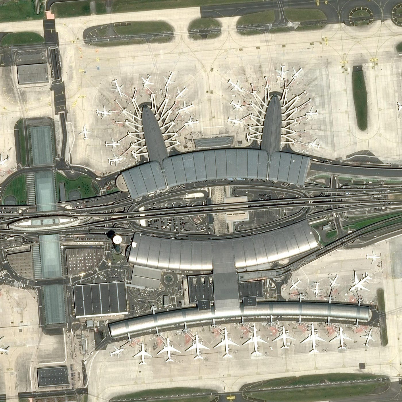
Looking at satellite images of airports can be pretty fascinating. You can see all of the different buildings and airstrips and get a sense of how busy the airport is. But did you know that you can also learn a lot about the activity of an airport by automatically monitoring the location and type of aircrafts?
Annotations Link to heading
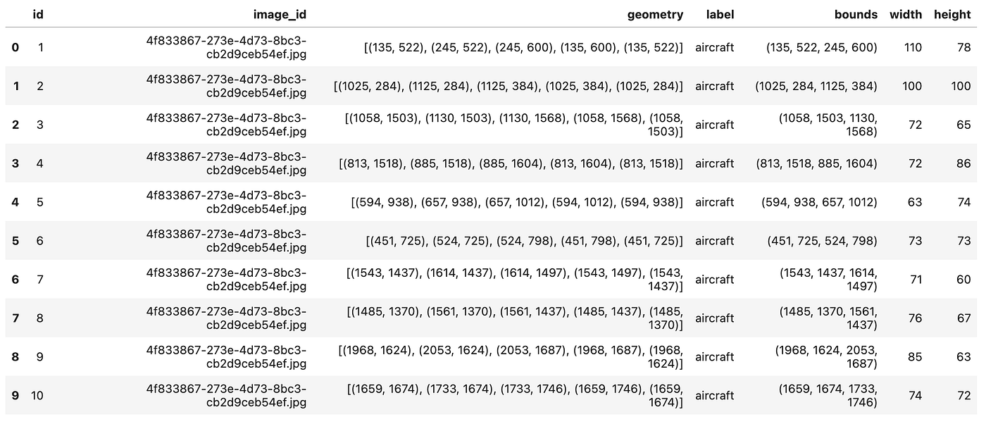
The annotations file contains a list of all the aircrafts visible on the images with the id of the associated image, a list of coordinates describing the outer boundaries of the aircraft and a label, usually Aircraft and sometimes Truncated_aircraft .
Here we will convert the geometries to bounding boxes as this is the usual format for detection models and replace the two categories by only aircraft.
Tilling Link to heading
The images available in the dataset are too large to fit into GPU memory at full resolution. We do not want to resample them because we do not want to loose small details in the images. So the following code cut the 2560x2560 images into several smaller 512x512 tiles. We select this pretty small size because we want to be able to fit more than one tile on the GPU in order to maintain a reasonable batch_size. But we also make sure that the size is large enough to fit most planes. In our case, 512 x 0.5 m/pix. is 128 meters which is larger than most planes’ wingspan.
We subsequently process the annotation DataFrame by associating each annotations with its tile_id as well as its image_id.
Note: here we do not use the parameter to generate an overlap between the tiles. This is because the train/val split is done later on by an IceVision helpers which works on the tiles and not on the source imagery. If we had left an overlap, some areas from the same source image could be in the train and in the validation dataset. This would lead to a leak which would impact training as validation would not contain only not previously seen data.
Check source code for tiling in:
https://www.kaggle.com/code/jeffaudi/aircraft-detection-with-yolov5
Deterministic behavior Link to heading
Our objective is to compare various deep learning architectures. So, we are going to train various architectures and compare the results (i.e. the best loss and best metric). In order for these comparaisons to be fair, we need to make sure that our training is deterministic. So we want to make sure that all random numbers used in functions (such as splitting between train and valid dataset) always return the same value. The following function will make sure that all sources of randomness are seeded with the same number every time.
def seed_everything(s=42):
    random.seed(s)
    os.environ['PYTHONHASHSEED'] = str(s)
    np.random.seed(s)
    torch.manual_seed(s)
    #imgaug.random.seed(s)

    if torch.cuda.is_available():
        torch.cuda.manual_seed(s)
        torch.cuda.manual_seed_all(s)
        torch.backends.cudnn.deterministic = True
        torch.backends.cudnn.benchmark = False

SEED = 42
seed_everything(SEED)
This function is pretty simple so it will not seed the workers (i.e. sub-processes). So, we will define num_workers to 0 so that we use only the main thread. We will loose in speed but this is not an issue now because we just want to figure which is the best architecture for this task.
IceVision Parser Link to heading
Next, we need to write an IceVision Parser. This is one of the most magical piece of code in IceVision. It enables to smoothly use our content in PyTorch data loaders and subsequently in Fastai or Pytorch Lightning. Here is the functions that we need to implement to create an IceVision Parser.
class MyParser(Parser):
    def __init__(self, template_record):
        super().__init__(template_record=template_record)

    def __iter__(self) -> Any:

    def __len__(self) -> int:

    def record_id(self, o: Any) -> Hashable:

    def parse_fields(self, o: Any, record: BaseRecord, is_new: bool):
        record.set_img_size(<ImgSize>)
        record.set_filepath(<Union[str, Path]>)
        record.detection.set_class_map(<ClassMap>)
        record.detection.add_labels(<Sequence[Hashable]>)
        record.detection.add_bboxes(<Sequence[BBox]>)
Hopefully, if you have a Pandas DataFrame, it is pretty straightforward.
class AirbusAircraftParser(Parser):
    def __init__(self, template_record, df):
        super().__init__(template_record=template_record)

    self.df = df
    self.class_map = ClassMap(list(self.df['label'].unique()))

    def __iter__(self) -> Any:
        for o in self.df.itertuples():
            yield o

    def __len__(self) -> int:
        return len(self.df)

    def record_id(self, o) -> Hashable:
        return o.tile_id

    def parse_fields(self, o, record, is_new):
        if is_new:
            record.set_filepath(TILES_PATH / o.tile_id)
            record.set_img_size(ImgSize(
               width=TILE_WIDTH, height=TILE_HEIGHT))
            record.detection.set_class_map(self.class_map)

        record.detection.add_bboxes([BBox.from_xyxy(
          o.x_min, o.y_min, o.x_max, o.y_max)])
        record.detection.add_labels([o.label])
Then, we can create a AirbusAircraftParser object and check that we get the correct classes for out task.
# here we create the parser for the Airbus aircraft dataset
parser = AirbusAircraftParser(TEMPLATE_RECORD, tiles_df)

# we check the number and name of classes
print(parser.class_map)
<ClassMap: {'background': 0, 'aircraft': 1}>
Next, we will use the parse() function to split the records into a train and a validation sets with respectively 80% and 20% of elements. We define the SEED to make sure that we have consistent train and valid sets between runs.
seed_everything(SEED)
train_records, valid_records =
    parser.parse(RandomSplitter([0.8, 0.2], seed=SEED))
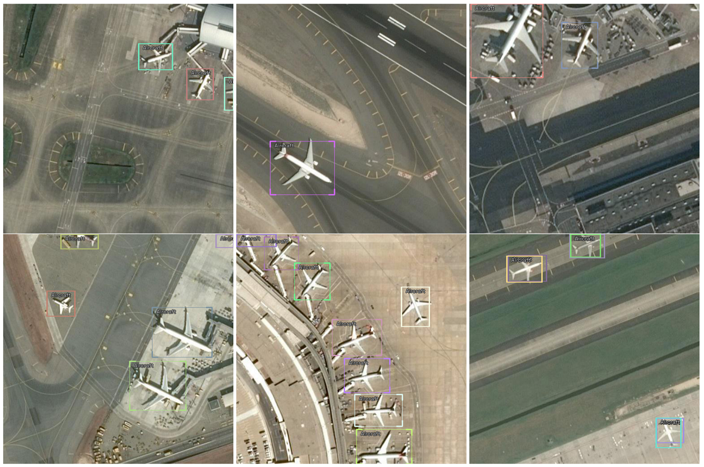
The parser() function also take care of correcting and removing incorrect records (typically points which may be outside of the imagery). Next, we can display some records with just one line of code!

# let's display some records!
show_records(random.choices(train_records, k=6), ncols=3)
Transformations Link to heading
The purpose of using transformations is to programmatically increase the number of images used to train the network. Too few images will cause the model to overfit quickly (i.e. learn to replicate exactly the training data). By applying transformations to the training data, we ensure that we can use larger backbones and longer training time — globally improving the models while avoiding overfitting.
IceVision integrates the[imgaug](https://github.com/aleju/imgaug) library which is especially suited for detection tasks because it is able to augment the image as well as the associated annotations. It is also nice to augment to use on satellite images because it has such a variety of augmentation (and even weather augmenters like fog or clouds).
Here, we will be using a very basic set of augmentation which works well for satellite images and apply them only on the training dataset.
# seed everything
seed_everything(SEED)

# define some transformation adapted to satellite imagery
train_tfms = tfms.A.Adapter([
    tfms.A.VerticalFlip(p=0.5),
    tfms.A.HorizontalFlip(p=0.5),
    tfms.A.Rotate(limit=20),
    tfms.A.GaussNoise(p=0.2),
    tfms.A.RandomBrightnessContrast(p=0.2),
    tfms.A.Normalize(),
])

# no transformation on the validation split
valid_tfms = tfms.A.Adapter([tfms.A.Normalize()])
Next, we just need to create the PyTorch datasets from the records.
# we create the train/valid Dataset objects
train_ds = Dataset(train_records, train_tfms)
valid_ds = Dataset(valid_records, valid_tfms)
Model architecture Link to heading
And this is where the magic happens! By leveraging the IceVision integration layers, we are able to easily access hundreds of neural net architectures and backbones.
In the article, we will just test 4 different models with different backbones
- RetinaNet (with ResNet-34 or ResNet-50 backbones)
- FasterRCNN (with ResNet-34 or ResNet-50 backbones)
- EfficientDet (with two small backbones)
- YOLOv5 (with small backbone)
Here we define a model name which integrates the name of the library (torchvision, ross, mmdet, ultralytics, etc.), the name of the architecture (retinanet, faster_rcnn, yolov5, etc.) and the name of the backbone (resnet34, resnet50, d0, etc.)
# the selected architecture
SELECTION = 3

# default parameters
BATCH_SIZE = 16
extra_args = {}

if SELECTION == 1:
    model_name = "torchvision-retinanet-resnet34_fpn"

elif SELECTION == 2:
    model_name = "torchvision-retinanet-resnet50_fpn"

elif SELECTION == 3:
    model_name = "torchvision-faster_rcnn-resnet34_fpn"

elif SELECTION == 4:
    model_name = "torchvision-faster_rcnn-resnet50_fpn"

elif SELECTION == 5:
    model_name = "ross-efficientdet-tf_lite0"
    extra_args['img_size'] = image_size

elif SELECTION == 6:
    model_name = "ross-efficientdet-d0"
    extra_args['img_size'] = image_size

elif SELECTION == 7:
    model_name = "ultralytics-yolov5-medium"
    extra_args['img_size'] = image_size
The extra_args dictionary will enable to add parameters specific to the architecture. We can for example also change the batch_size based on the architecture.
We can retrieve an pointer on the model that we have selected. This is actually an IceVision adaptator on the model from the corresponding library.
# seed everything
seed_everything(SEED)

tokens = model_name.split("-")
library_name = tokens[-3]
print(f"Library name: {library_name}")
arch_name = tokens[-2]
print(f"Architecture name: {arch_name}")
backbone_name = tokens[-1]
print(f"Backbone name: {backbone_name}")

model_type = getattr(getattr(models, library_name), arch_name)
backbone = getattr(model_type.backbones, backbone_name)

model = model_type.model(backbone=backbone(pretrained=True),
	num_classes=len(parser.class_map), **extra_args)
The magic here is that the model is coming from various libraries but still integrates seamlessly with the IceVision API. The following code is the same for any of the previously selected models. Here, we create the data loaders and display the first batch.
Note that we are passing _num_workers=0_ to avoid using sub-processes in data loaders as this generates an extra complexity to pass the random seed to sub-processes.
# we create the train/valid DataLoaders objects
train_dl = model_type.train_dl(train_ds,
batch_size=BATCH_SIZE, num_workers=0, shuffle=True)
valid_dl = model_type.valid_dl(valid_ds,
batch_size=BATCH_SIZE, num_workers=0, shuffle=False)
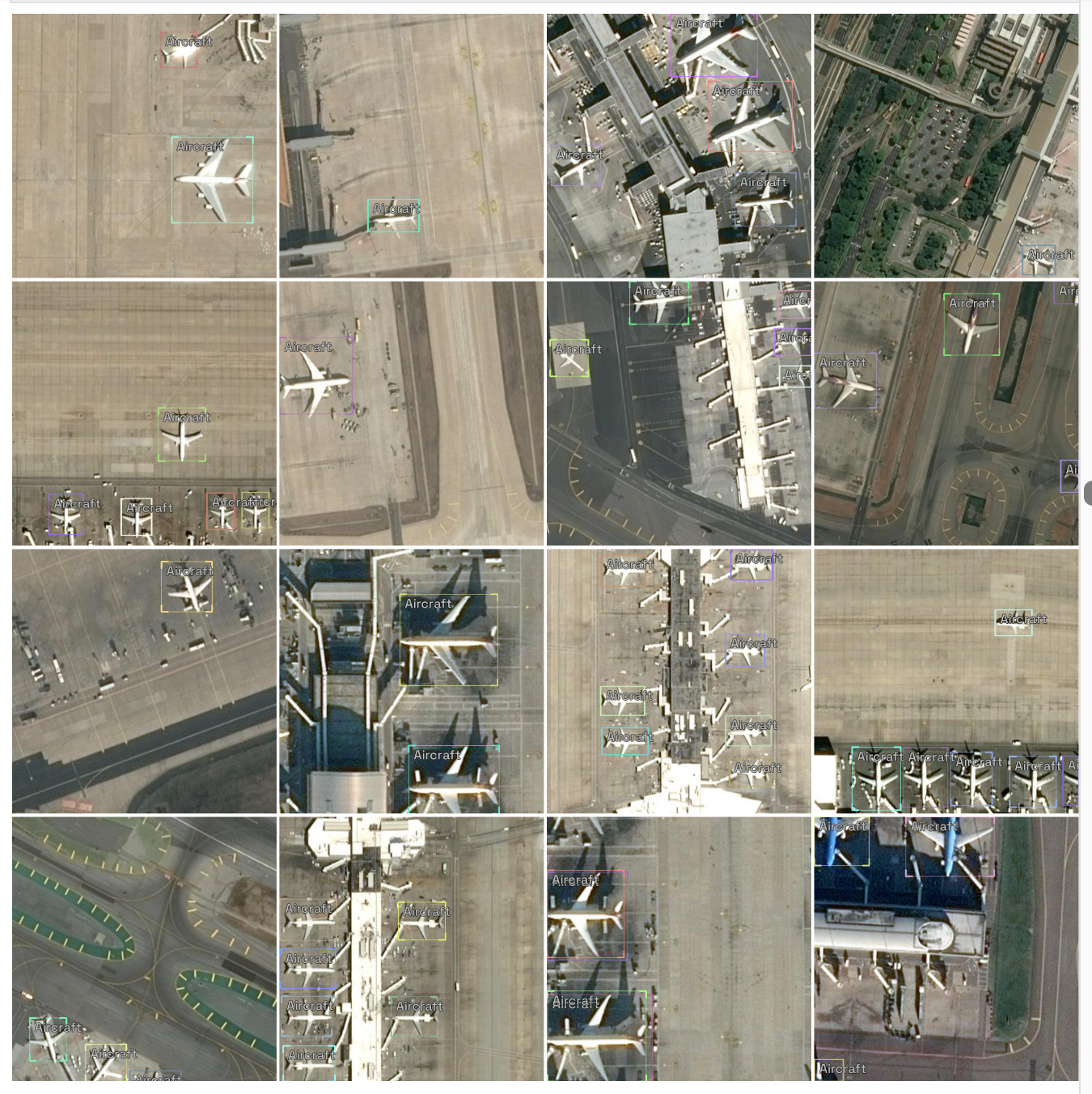
# display the first batch for checking
model_type.show_batch(first(valid_dl), ncols=4)
Finding the optimal learning rate Link to heading
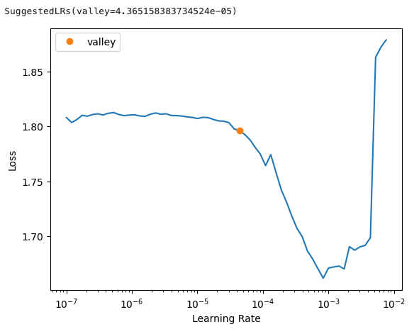
Each deep learning architecture as well as each backbone has its own ideal learning rate. Fastai has a cool feature to find the optimal learning rate. Here, we will define the metric that we want to use for validation and create a fastai learner. This object has a lr_find() function which will run training iterations while slightly increasing the learning rate. It will compute an ideal learning rate after
metrics = [COCOMetric(metric_type=COCOMetricType.bbox)]
learn = model_type.fastai.learner(dls=[train_dl, valid_dl],
            model=model, metrics=metrics)
learn.lr_find()
These is a typical output of the lr_find() function. The suggested LR is selected to be large enough to decrease the loss at each iteration without generating a gradient explosion (i.e. overshooting the minima and generating always increasing values for the loss).
After running lr_find() for all architectures, we can define the initial learning rate depending of the current selection, as follows:
if SELECTION == 1 or SELECTION == 3:
    LR = 1e-4
elif SELECTION == 2 or SELECTION == 4:
    LR = 5e-5
else:
    LR = 0.001

print(f"Model is {model_name}")
print(f"Learning rate is {LR}")
Training Link to heading
For the sake of demonstration, we will now use PyTorch Lightning to train our models. We can move easily from one library to another depending on our needs.
This is the minimum code that we need:
class LightModel(model_type.lightning.ModelAdapter):
    def configure_optimizers(self):
        return Adam(self.parameters(), lr=LR)

MAX_EPOCHS = 10
trainer = pl.Trainer(max_epochs=MAX_EPOCHS, accelerator='gpu',
          devices=1, log_every_n_steps=10)

trainer.fit(light_model, train_dl, valid_dl)
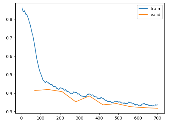
We can control that the training loss (blue) and validation loss (orange) are going down with iterations. The training loss decrease in a very regular manner whereas the validation loss is a little more bumpy but still gradually decreasing.
Computing the final metric Link to heading
To compute the final metric, we will create a new PyTorch Lightning trainer to make sure that we have a clean state and use the test() function.
# compute the final metric with the same trainer
#results = trainer.validate(dataloaders=valid_dl, verbose=True)

# testing model with a new trainer
seed_everything(SEED)
valid_dl = model_type.valid_dl(valid_ds,
        batch_size=BATCH_SIZE, num_workers=0, shuffle=False)

trainer = pl.Trainer(accelerator='gpu', devices=1)
results = trainer.test(light_model, valid_dl)
After running the training and testing multiple times, here are the results for each architecture:

Despite our seed_everything(SEED) function to make sure that we have a deterministic behavior, Faster-RCNN and YOLOv5 still delivered different final metrics. For Faster-RCNN, it seems that RoIAlign() uses atomicAdd() on the GPU, which breaks determinism even if all flags and seeds are set correctly. A similar issue is probably also the reason why YOLOv5 is not deterministic either. The other architectures always delivered the exact same final metric for each run.
Analysis Link to heading
Takeout #1 Link to heading
The best architectures for this task are Faster-RCNN and EfficientDet. It is important to mention that this is only for this task because there is a lot of difference between earth observation tasks. Aircraft detection, vehicle detection (much smaller objects) and crop identification (use of channels and time series) are very different tasks. On top of this, there is not a single dataset that we can use to be a universal dataset for benchmarking such as Microsoft COCO for object detection.
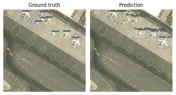
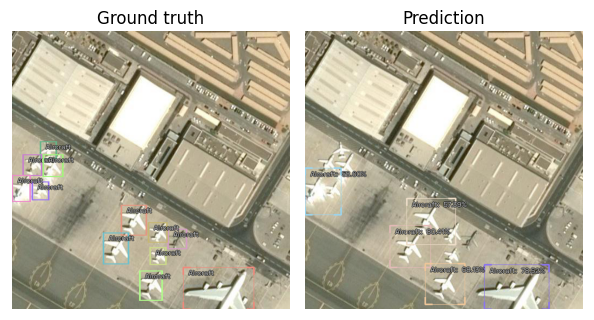
We can visualize the detections by using the following code:
model_type.show_results(model, valid_ds, detection_threshold=.30)
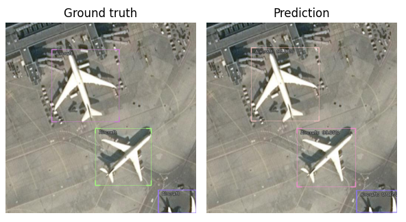
The detections are very good with the model being able to detect planes even at the edge of the tiles. This definitely leads to issues like on this following case.
The sky bridge is detected as a plane and this is interesting because there is often a sky bridge close to a parked aircraft. We will need to make sure that we have enough empty parking spots with sky bridges and no aircrafts in the training database.
Takeout #2 Link to heading
It seems that small backbones like ResNet-34 are already able to understand our task. Faster-RCNN does not perform much better with a ResNet-50 backbone rather than a ResNet-34.
Smaller backbones are quicker to train and are lighter and faster for inference. On a larger dataset, with a more complex task such as identifying type of aircrafts, we might need to increase the size of the backbone but for this task and this dataset, ResNet-34 seems to be good enough.
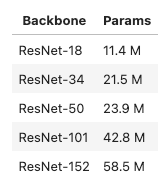
By quickly training with Faster-RCNN and a ResNet-18 backbone we can confirm that ResNet-18 is not enough to correctly understand the task with under 10 epochs.
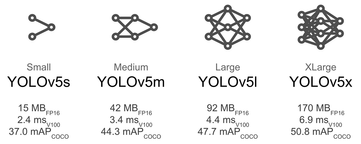
YOLOv5-m has 20.9 M parameters which is similar to ResNet-34. This is why we have selected this architecture rather than YOLOv5-s which has only 7.5 M parameters. Like ResNet-18, YOLOv5-s is too small to learn correctly the task in less than 10 epochs.
EfficientDet is doing very well on the task even with a very small number of parameters compared to the other models (typically less than 4 M parameters). There is not much difference between the two architectures. The main difference is that tf_lite0 are weights trained with TensorFlow and ported to PyTorch whereas d0 are weights trained natively on PyTorch EfficientDet by Ross Wightman.
Takeout #3 Link to heading
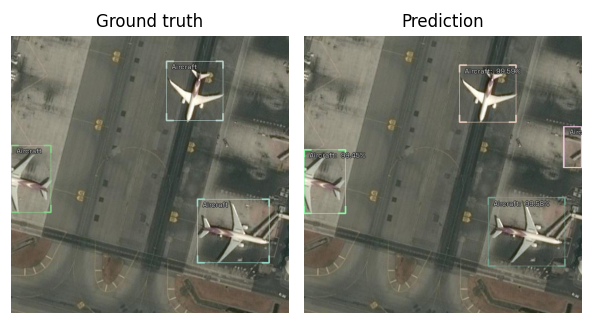
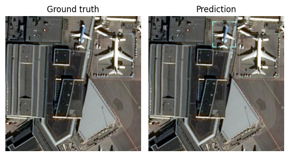
RetinaNet seems doing pretty bad on this task. To understand why, we can visualize the results by using the following code:
model_type.show_results(model, valid_ds, detection_threshold=.15)
As we can see above, the model has missed one aircraft and has provided many predictions for the same aircrafts. This is definitely bringing the accuracy down as the COCO metric associate one prediction with only one ground truth — the other predictions being considered false alerts. Many predictions for the same object is not abnormal for detection architectures but is usually cleared by the use of NMS — Non-Maximal-Suppresion. There is typically such an issue in our RetinaNet model, either in the code itself or in the selected hyper-parameters for NMS.
To dive deeper, we can also use a specific IceVision object called interp which is inspired by a similar object in Fastai. The interp object helps to understand model behavior and has a specific function plot_top_losses() that could be used to display the objects with the greatest losses. This usually shows where the models fails and helps understanding why.
samples_plus_losses, preds, losses_stats =
	model_type.interp.plot_top_losses(model=model,
		dataset=valid_ds, sort_by="loss_total", n_samples=6)
In this case, we see that one aircraft has been missed in the ground truth. This is definitely penalize all models. This is a good example how the qualification dataset needs to be very accurate in order to correctly asses the quality of the model.

In the above example, we see that the model does not detect the tail of the aircraft that is visible at the bottom of the tile. It shows how the parameter to keep or delete truncated objects need to be carefully selected. In our case, we selected TRUNCATED_PERCENT = O.3 but this percentage is computed for the horizontal box which is not always coherent with the visible features of the object to detect (aircrafts do not fill the horizontal bounding boxes).
Finally, the above example is clearly showing the difficulties of the model to detect small aircrafts. This is probably linked to the size of the predefined anchors.

With YOLOv5-m, the model is still confused with sky bridges and even airport buildings after 10 epochs. This is probably due to non optimal anchor sizes and smaller objects than usually in the COCO dataset. I am definitely surprised by this as I have used YOLOv3 and YOLOv5 successfully for this task. I have even written an article on this topic in 2021. In the article, I only do 10 epochs as well and get good results. Maybe we should dig into the integration of YOLOv5 in IceVision?
Conclusion Link to heading
We just showed that EfficientDet and Faster-RCNN are performing well after a few epochs of training when qualified over this small sample Airbus Aircraft detection dataset. EfficientDet has 5 times less parameters and should be preferred for production since less parameters means faster inference time (and lower cost if you are using it on the cloud).
It does not mean that they will always be the best models. Each task and each sensor is different (especially with regard to resolution and spectral bands). And let me also remind here that the dataset that we used is by no means a good qualification dataset.
My main objective here was to demonstrate that IceVision is a very nice framework to check on your specific dataset and your specific task which are the most promising models.
Once your model and architecture selected, you might want to continue to use IceVision or switch to the source implementation (i.e. Torchvision, Ultralytics, MMLab, etc.) for production and deployment. There will still be a lot of work to be done on the hyper-parameters, the training process and on the dataset itself to produce a final high performance detector.
If you like this post, please clap for it, follow me and read my other articles:
- Oil Storage Detection on Airbus Imagery with YOLOX
- Detecting aircraft on Airbus Pleiades imagery with YOLOv5
- Things you should know before organizing a Kaggle Competition
And finally, if you want to dive more into the code, here is a link to the notebook that I created to write this article.
Written on January 2, 2023 by Jeff Faudi.
Originally published on Medium