Introduction Link to heading
Last year, Airbus Intelligence published a few Machine Learning Datasets on the Kaggle platform. These datasets are samples from much larger and more comprehensive datasets provided by Airbus. Nevertheless, they are good datasets to start with and build upon if you wish to learn more about Earth Observation imagery and Deep Learning.
In this article, we will analyse the Airbus Oil Storage dataset. It contains one hundred SPOT images and a little over 13,500 annotated POL (Petroleum, Oil and Lubricant) storage. Using this dataset, we can train an Oil Storage detector based upon the YOLO series. We will test YOLOv3 and YOLOv5 versions based on the implementation from Ultralytics [coming soon] as well as YOLOX version based on the implementation from Megvii.
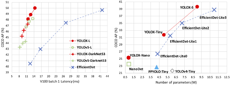
Although these implementation share the YOLO name, there are all very different beasts. YOLOX is an anchor-free version of YOLO, with a simpler design but better performance! It aims to bridge the gap between research and industrial communities. For more details, you can check the report on Arvix: YOLOX: Exceeding YOLO Series in 2021.
If you want to look at some code, you can follow along with the associated Kaggle notebooks:
With inspiration from and credits to:
- https://www.kaggle.com/code/regonn/airbus-oil-storage-detection-simple-yolox/notebook
- https://www.kaggle.com/remekkinas/yolox-training-pipeline-cots-dataset-lb-0-507
Dataset analysis Link to heading
The dataset contains 98 JPEG images. The images are actually 2560 pixels by 2560 pixels images in RGB (3 bands) in JPEG format. They are extracted from the SPOT archive and provided at a resolution of 1.50 meter per pixel. They come from various locations all over the Earth.
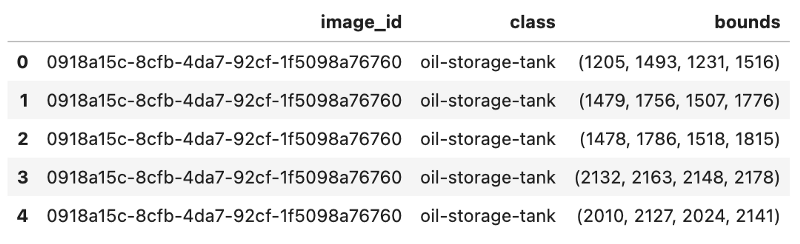
The annotations are provided as a CSV file with reference the image, geometry as a closed polygon, and class. There are 13,592 annotations for oil storage tanks.
Some images contain only a few annotations while other images can count more than several hundreds. As a matter of fact, there are 4 images with less than 20 annotations and also 4 images with more than 400 annotations.
Let’s display the distribution of annotations per image:
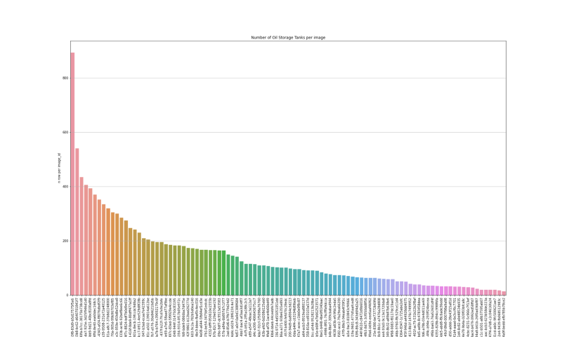
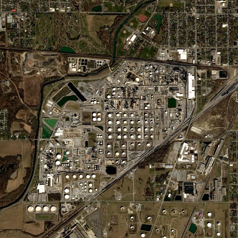
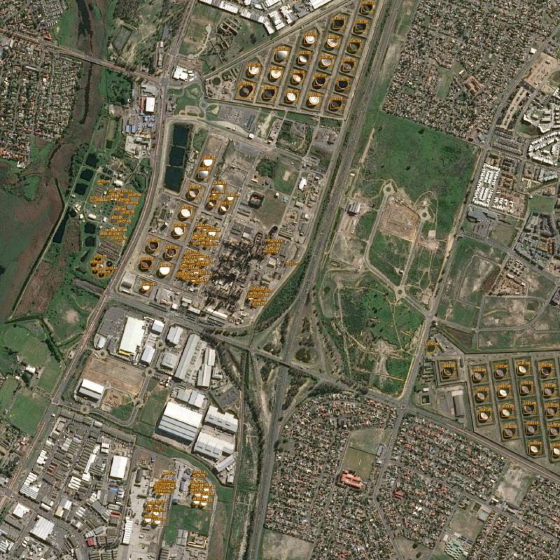
One image as almost 900 annotations (893 actually). We can display it with its annotations to check that there was now issue with the labelling.
It seems pretty much okay! Note that oil storage tanks have very different kind of sizes. And also that the smallest ones, with a few pixels width might already around 6 meters wide at 1.5 meter/pixel.
Apart from this one, the rest of the dataset is well balanced with an evenly distributed number of annotation per image.
From the bounding boxes, we can compute the width and height (which should be very similar) and display some statistics:
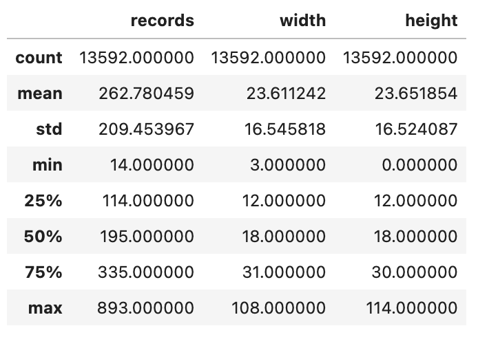
Here we can confirm that height and width are pretty much correlated which is a good sign. The minimum of zero for the height is an indication that we have probably some mis-labelled objects.
We can display the distribution of width and height of bounding boxes.
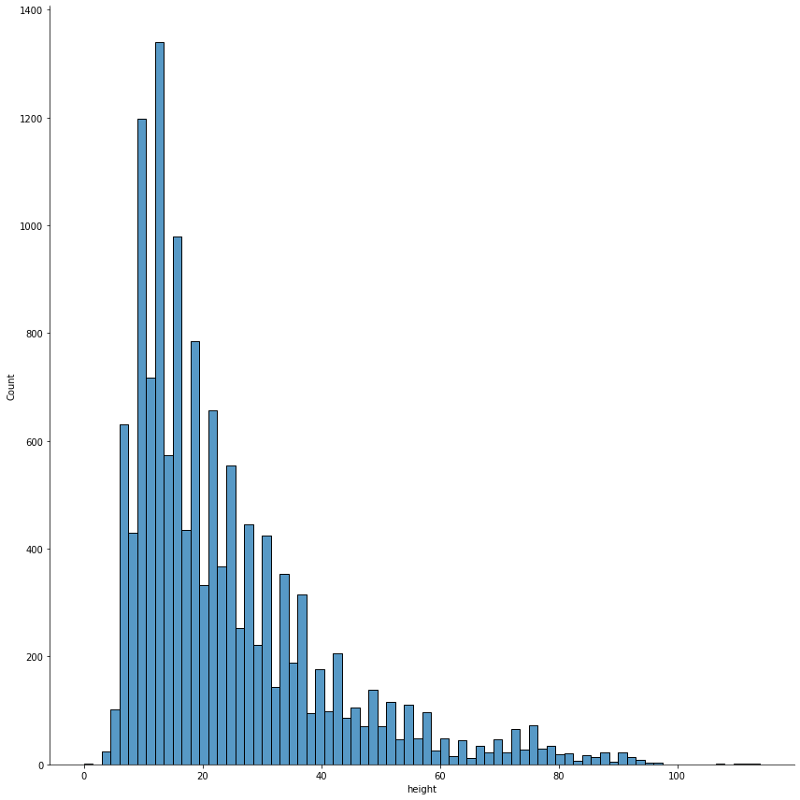
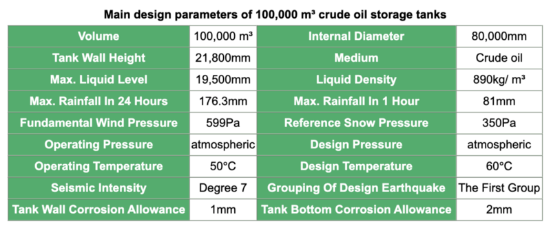
This seems correct with typical diameter of 10 pixels i.e. 15 meters for the small storages. The typical diameter for a large oil storage tanks seems to be around 80 meters. The largest ones with a capacity of 250,000 m3 should have a diameter of 120 meters i.e. 80 pixels. The storages with a width above this limit are probably not very well labelled due to the angle of view which could add an extra 20 to 30 meters.
One other interesting aspect of this histogram is the way that high and low measurements are interlaced. One explanation of this artefact could be that the tool used to create the annotation would favor even number of pixels over odd number of pixels. If you have another explanation, please get back to me or use the comment section.
The next step would be to compute the aspect ratio of the oil storage. We expect a mean value of 1.0 with a very small deviation.
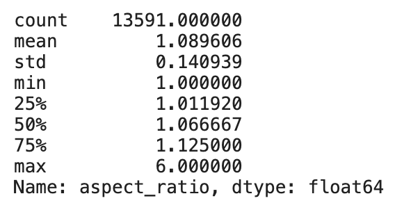
Actually 75% of the objects have an aspect ratio under 1.125 but some outliers are stretching the metric. These are probably oil storage truncated at the border of the imagery.
In the following steps, we have decided to remove small objects under 5 pixels width as well as objects with an aspect ratio larger than 2.5. This results in removing 50 records which are too small and 21 records with too large aspect ratio. This is only 71 annotations over 13,592 total.
Training YOLOX Link to heading
In this article, we will use the YOLOX version based on the implementation fromMegvii. Please visit these above link for more information.
The images are too big to be used directly in the training. On a standard GPU, we will not be able to load more than one or two images. But we need regularization to train our model well, so we need to use a batch size of 16 or even better 32 samples. This will not work with such large images; we need to make smaller images (or tiles).
But before doing this, we will create the splits between training, validation and test. We want to do this before tiling so that all tiles from the same image end up in the same split. Otherwise we will create leaks between the training, validation and test splits (especially because we will generate overlaps between the tiles).
# Percentage to allocate to train, validation and test datasets
train_ratio = 0.75
valid_ratio = 0.15
test_ratio = 0.10
Next, we generate the tiles on disk with a selected size of 512 pixels by 512 pixels. In order to make sure that every aircraft can be seen by the network in full, we allow for an overlap of 64 pixels between the tiles. And we generate the tiles in the folder /kaggle/working. You can find the code in the Kaggle notebook.
# Create 640 x 640 tiles with 64 pix overlap in /kaggle/working
TILE_WIDTH = 640
TILE_HEIGHT = 640
TILE_OVERLAP = 64
TRUNCATED_PERCENT = 0.3
This will generate a lot of truncated objects but the network will be able to detect the truncated oil storages if enough of it is visible. So, we will remove the annotation only if there is less than 30% of the bounding box left visible on the image.
YOLOX uses the COCO file format. So while we generate the tiles on disk, we also generate the associated COCO files as follows:
- Train folder contains 1,825 tiles and 14,316 annotations
- Validation folder contains 375 tiles and 2,281 annotation
- Test folder contains 250 tiles and 1,664 annotations
After creating a few more configuration files (check the Kaggle notebook), we are able to launch a training of YOLOX on our data. We start with the YOLOX-s model weights for now.
After 10 epochs, the output is the following:
Average Precision  (AP) @[ IoU=0.50:0.95 | area=   all] = 0.588Average Precision  (AP) @[ IoU=0.50      | area=   all] = 0.856Average Precision  (AP) @[ IoU=0.75      | area=   all] = 0.667

Average Precision  (AP) @[ IoU=0.50:0.95 | area= small] = 0.500Average Precision  (AP) @[ IoU=0.50:0.95 | area=medium] = 0.802Average Recall     (AR) @[ IoU=0.50:0.95 | area=   all] = 0.633Average Recall     (AR) @[ IoU=0.50:0.95 | area= small] = 0.554Average Recall     (AR) @[ IoU=0.50:0.95 | area=medium] = 0.847
So, after a few epochs and no specific tuning, we already get a recall of 85% for large oil storage. For smaller oil storages, the recall is just above 55%.
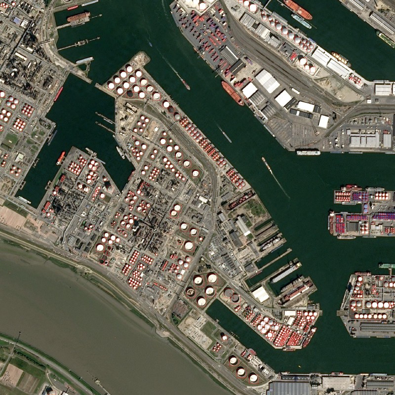
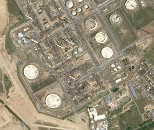
We also get an **average precision over 80%**for large oil storage over IoU between 0.50 and 1.0. As we can see in the following image, these are typically other round structures such as water processing tanks which are incorrectly detected as oil storage (i.e. false alarms).
Of course, this can be improved but seems pretty good already. We can run some predictions on the sample imagery and display them. Here is one:
Next steps Link to heading
The obvious next steps are to train for more epochs and potentially tag the mis-predicted objects (such as water treatment tanks) to sample them more often and improve the precision of the model.
Another next step is clearly to improve the dataset by including more images and more diversity. You can do this by hand or by running your new detector on archive satellite imagery. You can also look into new innovative ways like using synthetic data to improve your detector.
Remember that the Airbus dataset is provided under a Creative Commons BY-NC-SA license. So, this is mostly to learn, test and share with friends, students and colleagues. It cannot be used in commercial applications. If you want more imagery and licence rights, visit the Airbus OneAtlas platform.
You can also learn how to publish your inference code as a Docker container and host it on an analytics platform like UP42. You can copy some boilerplate code from UP42 Github and follow along with their documentation. This will enable you to run your algorithm at scale on some fresh imagery.
If you enjoyed this story, please clap and follow me for more.
Written on June 15, 2022 by Jeff Faudi.
Originally published on Medium